Modeling Examples

This chapter includes commented mip.examples on modeling and solving optimization problems with Kotlin-MIP.

The 0/1 Knapsack Problem

As a first example, consider the solution of the 0/1 knapsack problem: given a set \(I\) of items, each one with a weight \(w_i\) and estimated profit \(p_i\), one wants to select a subset with maximum profit such that the summation of the weights of the selected items is less or equal to the knapsack capacity \(c\). Considering a set of decision binary variables \(x_i\) that receive value 1 if the \(i\)-th item is selected, or 0 if not, the resulting mathematical programming formulation is:

\[\begin{split}\textrm{Maximize: } \;\;\; & \sum_{i \in I} p_i \cdot x_i \\ \textrm{Subject to: } \;\;\; & \sum_{i \in I} w_i \cdot x_i \leq c \\ & x_i \in \{0,1\} \,\,\, \forall i \in I\end{split}\]

The following kotlin code creates, optimizes and prints the optimal solution for the 0/1 knapsack problem. To make the code easier to read, we use alias functions list and sum, but we could replace them by kotlin’s map function.

Solves the 0/1 knapsack problem: Knapsack.kt

import mip.*

fun main() {
    // problem's input data
    val p = arrayOf(10, 13, 18, 31, 7, 15)
    val w = arrayOf(11, 15, 20, 35, 10, 33)
    val c = 47
    val I = w.indices // 0 until w.size

    // creating model
    val m = Model("Knapsack", solverName = GUROBI)
    m.verbose = false

    // creating vars and setting objective function
    val x = I.map { i -> m.addBinVar("item_$i") }
    m.objective = maximize(I.sum { i -> p[i] * x[i] })

    // adding constraint and solving model
    m += I.sum { i -> w[i] * x[i] } leq c
    m.optimize()

    // printing result
    val selected = x.filter { it.x >= 0.99 }
    println("Total cost: ${m.objectiveValue}")
    println("Selected items: $selected")
}

Line 3 imports the required classes and definitions from Kotlin-MIP. Lines 5-8 define the problem data. Line 11 creates an empty maximization problem m with the (optional) name “Knapsack”. Line 14 adds the binary decision variables to model m and stores their references in a collection x. Line 15 sets the objective function, and line 18 adds the capacity constraint (using the operator leq, indicating \(\leq\)). The model is optimized in line 19 and, finally, the solution is computed and printed by lines 22-23. Note that we use kotlin’s filter function to make the code shorter (and more readable).

The Traveling Salesman Problem

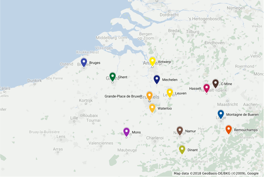
The traveling salesman problem (TSP) is one of the most studied combinatorial optimization problems, with the first computational studies dating back to the 50s [Dantz54], [Appleg06]. In order to illustrate this problem, consider that you will spend some time in Belgium and wish to visit some of its main tourist attractions, depicted in the map bellow:

You want to find the shortest possible tour to visit all these places. More formally, considering \(n\) points \(V=\{0,\ldots,n-1\}\) and a distance matrix \(D_{n \times n}\) with elements \(c_{i,j} \in \mathbb{R}^+\), a solution consists of a set of exactly \(n\) (origin, destination) pairs indicating the itinerary of your trip, resulting in the following formulation:

\[\begin{split}\textrm{Minimize: } \;\;\; & \sum_{i \in V, j \in V} c_{i,j} \ldotp x_{i,j} \\ \textrm{Subject to: } \;\;\; & \sum_{j \in V \setminus \{i\}} x_{i,j} = 1 \,\,\, &\forall i \in V \\ & \sum_{i \in V \setminus \{j\}} x_{i,j} = 1 \,\,\, &\forall j \in V \\ & y_{i} -(n+1)\ldotp x_{i,j} \geq y_{j} -n \;\;\,\,\, &\forall i \in V\setminus \{0\}, j \in V\setminus \{0,i\}\\ & x_{i,j} \in \{0,1\} \,\,\, &\forall i \in V, j \in V \\ & y_i \geq 0 \,\,\, &\forall i \in V\end{split}\]

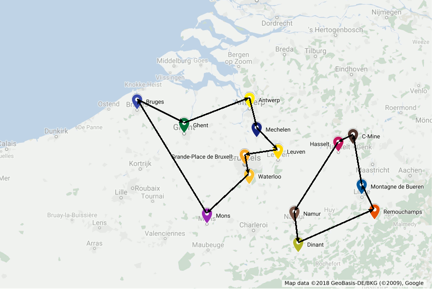
The first two sets of constraints enforce that we leave and arrive only once at each point. The optimal solution for the problem including only these constraints could result in a solution with sub-tours, such as the one presented bellow:

To enforce the production of connected routes, additional variables \(y_{i} \geq 0\) are included in the model to indicate the sequential order of each point in the produced route. Point zero is arbitrarily selected as the initial point and conditional constraints linking variables \(x_{i,j}\), \(y_{i}\) and \(y_{j}\) are created for all nodes except the initial one to ensure that the selection of an arc \(x_{i,j}\) implies that \(y_{j}\geq y_{i}+1\).

The kotlin code to create, optimize and print the optimal route for the TSP is included bellow. Note that we employ functions map and filter from kotlin’s standard library again.

Traveling salesman problem solver with compact formulation: TSPCompact.kt

import mip.*

fun main() {
    // names of places to visit
    val places = arrayOf(
        "Antwerp", "Bruges", "C-Mine", "Dinant", "Ghent", "Grand-Place de Bruxelles",
        "Hasselt", "Leuven", "Mechelen", "Mons", "Montagne de Bueren", "Namur",
        "Remouchamps", "Waterloo"
    )

    // distance matrix
    val c = arrayOf(
        arrayOf(0, 83, 81, 113, 52, 42, 73, 44, 23, 91, 105, 90, 124, 57),
        arrayOf(83, 0, 161, 160, 39, 89, 151, 110, 90, 99, 177, 143, 193, 100),
        arrayOf(81, 161, 0, 90, 125, 82, 13, 57, 71, 123, 38, 72, 59, 82),
        arrayOf(113, 160, 90, 0, 123, 77, 81, 71, 91, 72, 64, 24, 62, 63),
        arrayOf(52, 39, 125, 123, 0, 51, 114, 72, 54, 69, 139, 105, 155, 62),
        arrayOf(42, 89, 82, 77, 51, 0, 70, 25, 22, 52, 90, 56, 105, 16),
        arrayOf(73, 151, 13, 81, 114, 70, 0, 45, 61, 111, 36, 61, 57, 70),
        arrayOf(44, 110, 57, 71, 72, 25, 45, 0, 23, 71, 67, 48, 85, 29),
        arrayOf(23, 90, 71, 91, 54, 22, 61, 23, 0, 74, 89, 69, 107, 36),
        arrayOf(91, 99, 123, 72, 69, 52, 111, 71, 74, 0, 117, 65, 125, 43),
        arrayOf(105, 177, 38, 64, 139, 90, 36, 67, 89, 117, 0, 54, 22, 84),
        arrayOf(90, 143, 72, 24, 105, 56, 61, 48, 69, 65, 54, 0, 60, 44),
        arrayOf(124, 193, 59, 62, 155, 105, 57, 85, 107, 125, 22, 60, 0, 97),
        arrayOf(57, 100, 82, 63, 62, 16, 70, 29, 36, 43, 84, 44, 97, 0),
    )

    // number of cities (n) and range of them (V)
    val n = places.size
    val V = 0 until n

    val model = Model("TSPCompact")

    // binary variables indicating if arc (i,j) is used or not
    val x = V.list { i -> V.list { j -> model.addBinVar("x($i,$j)", obj = c[i][j]) } }

    // continuous variable to prevent subtours: each city will have a different
    // sequential id in the planned route (except the first one)
    val y = V.list { model.addNumVar("y($it)") }

    // Constraints 1 and 2: leave and enter each city exactly only once
    for (i in V) {
        model += V.filter { it != i }.sum { x[i][it] } eq 1 named "out_$i"
        model += V.filter { it != i }.sum { x[it][i] } eq 1 named "in_$i"
    }

    // Constraints 3: subtour elimination
    for (i in 1 until n)
        for (j in 1 until n) if (i != j)
            model += y[i] - n * x[i][j] geq y[j] - (n - 1)

    model.maxSeconds = 30.0
    model.optimize()

    // checking if a solution was found and printing it
    if (model.hasSolution) {
        println("Route with total distance ${model.objectiveValue} found:")
        var i = 0
        do {
            println("  - ${places[i]}")
            for (j in V) if (x[i][j].x >= 0.99) {
                i = j
                break
            }
        } while (i != 0)
    }
}

Lines 5-27 describe the problem, providing names for the places to visit and the distances between them. Lines 30-31 stores the number of nodes (n` and a range with nodes’ ids starting from 0 (V). In line 33 an empty MIP model is created. In line 36 all binary decision variables for the selection of arcs are created using function addBinVar and their references are stored in a \(n \times n\) matrix named x. Note that the objective function is defined while creating the variables: the argument obj (second argument of the function) indicates the coefficient of the variable in the objective function. We could, of course, create the objective function by setting property objective as well. In line 40, variables \(y\) are created. Note that, differently from \(x\) variables, \(y\) variables are not required to be binary or integral, and thus can be created using the addNumVar function.

Lines 42-51 we add constraints the constraints. We used operators eq (to represent equals), geq (equivalent to \(\geq\)) and the optional named to set the constraint’s names. In lines 49-51 we create the last set of constraints. In line 53 we set a runtime limit for the solver (30 seconds), and in line 54 we call the optimizer. The runtime limit will not be necessary for our Belgium example, which will be solved very quickly, but may be important for larger problems: even though high quality solutions may be found very quickly by the MIP solver, a long runtime may be required to prove optimality. With a time limit, the search is truncated and the best solution found during the search is reported. In line 57 we check for the availability of a feasible solution. Lines 58-67 print the route cost and all arcs selected in the route. Note that, again, we use the property x of a variable to query its value in the solution.

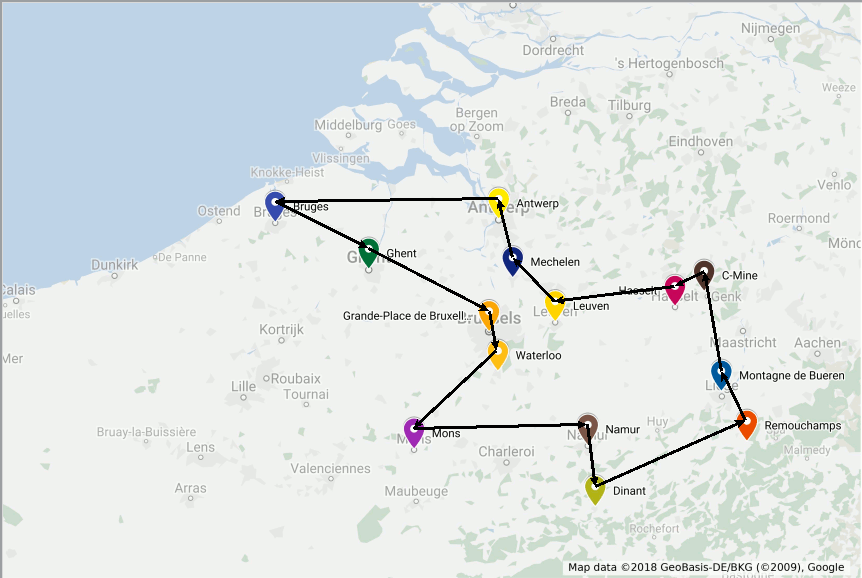
The optimal solution for our trip has length 547 and is depicted bellow:

n-Queens

In the \(n\)-queens puzzle \(n\) chess queens should to be placed in a board with \(n\times n\) cells in a way that no queen can attack another, i.e., there must be at most one queen per row, column and diagonal. This is a constraint satisfaction problem: any feasible solution is acceptable and no objective function is defined. The following binary programming formulation can be used to solve this problem:

\[\begin{split}\sum_{j=1}^{n} x_{ij} & = 1 \,\,\, &\forall i \in \{1, \ldots, n\} \\ \sum_{i=1}^{n} x_{ij} & = 1 \,\,\, &\forall j \in \{1, \ldots, n\} \\ \sum_{i=1}^n \sum_{j=1 : i-j=k}^{n} x_{i,j} & \leq 1 \,\,\, &\forall k \in \{2-n, \ldots, n-2\} \\ \sum_{i=1}^n \sum_{j=1 : i+j=k}^{n} x_{i,j} & \leq 1 \,\,\, &\forall k \in \{3, \ldots, n+n-1\} \\ x_{i,j} & \in \{0, 1\} \,\,\, &\forall i\in \{1, \ldots, n\}, j\in \{1, \ldots, n\}\end{split}\]

The following code builds the previous model, solves it and prints the queen placements:

Solver for the n-queens problem: Queens.kt

import mip.*

fun main() {
    // number of queens (n) and range of queens (ns)
    val n = 40
    val ns = 0 until n

    val queens = Model("nQueens")
    val x = ns.list { i -> ns.list { j -> queens.addBinVar("x($i,$j)") } }

    // one queen per row
    for (i in ns)
        queens += ns.sum { j -> x[i][j] } eq 1 named "row_$i"

    // one per column
    for (j in ns)
        queens += ns.sum { i -> x[i][j] } eq 1 named "col_$j"

    // diagonal \
    for (k in 2 - n .. n - 2) {
        val lhs = LinExpr()
        for (i in ns) if (i - k in ns)
            lhs += x[i][i - k]
        queens += lhs leq 1 named "diag1_${k.toString().replace("-", "m")}"
    }

    // diagonal /
    for (k in 3 .. n + n - 1) {
        val lhs = LinExpr()
        for (i in ns) if (k - i in ns)
            lhs += x[i][k - i]
        queens += lhs leq 1 named "diag2_$k"
    }

    queens.optimize()

    if (queens.hasSolution) {
        for (i in ns) {
            for (j in ns)
                print(if (x[i][j].x >= EPS) "O " else ". ")
            println()
        }
    }
}

Note that the formulation implemented above doesn’t have an objective function.

Frequency Assignment

The design of wireless networks, such as cell phone networks, involves assigning communication frequencies to devices. These communication frequencies can be separated into channels. The geographical area covered by a network can be divided into hexagonal cells, where each cell has a base station that covers a given area. Each cell requires a different number of channels, based on usage statistics and each cell has a set of neighbor cells, based on the geographical distances. The design of an efficient mobile network involves selecting subsets of channels for each cell, avoiding interference between calls in the same cell and in neighboring cells. Also, for economical reasons, the total bandwidth in use must be minimized, i.e., the total number of different channels used. One of the first real cases discussed in literature are the Philadelphia [Ande73] instances, with the structure depicted bellow:

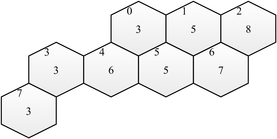
Each cell has a demand with the required number of channels drawn at the center of the hexagon, and a sequential id at the top left corner. Also, in this example, each cell has a set of at most 6 adjacent neighboring cells (distance 1). The largest demand (8) occurs on cell 2. This cell has the following adjacent cells, with distance 1: (1, 6). The minimum distances between channels in the same cell in this example is 3 and channels in neighbor cells should differ by at least 2 units.

A generalization of this problem (not restricted to the hexagonal topology), is the Bandwidth Multicoloring Problem (BMCP), which has the following input data:

\(N\):

set of cells, numbered from 1 to \(n\);

\(r_i \in \mathbb{Z}^+\):

demand of cell \(i \in N\), i.e., the required number of channels;

\(d_{i,j} \in \mathbb{Z}^+\):

minimum distance between channels assigned to nodes \(i\) and \(j\), \(d_{i,i}\) indicates the minimum distance between different channels allocated to the same cell.

Given an upper limit \(\overline{u}\) on the maximum number of channels \(U=\{1,\ldots,\overline{u}\}\) used, which can be obtained using a simple greedy heuristic, the BMPC can be formally stated as the combinatorial optimization problem of defining subsets of channels \(C_1, \ldots, C_n\) while minimizing the used bandwidth and avoiding interference:

\[\begin{split}\textrm{Minimize:} & \\ & \max_{c \in C_1 \cup C_2, \ldots, C_n}c \\ \textrm{Subject to:} & \\ \mid c_1 - c_2 \mid & \geq d_{i,j} \,\,\, \forall (i,j) \in N \times N, (c_1, c_2) \in C_i \times C_j \\ C_i & \subseteq U \,\,\, \forall i \in N \\ \mid C_i \mid & = r_i \,\,\, \forall i \in N\end{split}\]

This problem can be formulated as a mixed integer program with binary variables indicating the composition of the subsets: binary variables \(x_{(i,c)}\) indicate if for a given cell \(i\) channel \(c\) is selected (\(x_{(i,c)}=1\)) or not (\(x_{(i,c)}=0\)). The BMCP can be modeled with the following MIP formulation:

\[\begin{split}\textrm{Minimize:} & \\ & z \\ \textrm{Subject to:} & \\ \sum_{c=1}^{\overline{u}} x_{(i,c)} & = r_{i} \,\,\, \forall \, i \in N \\ z & \geq c\cdot x_{(i,c)} \,\,\, \forall \, i \in N, c \in U \\ x_{(i,c)} + x_{(j,c')} & \leq 1 \,\,\, \forall \, (i,j,c,c') \in N \times N \times U \times U : \, i \neq j \land \mid c-c' \mid < d_{(i,j)} \\ x_{(i,c} + x_{(i,c')} & \leq 1 \,\,\, \forall i,c \in N \times U, c' \in \{c,+1\ldots, \min(c+d_{i,i}, \overline{u}) \} \\ x_{(i,c)} & \in \{0, 1\} \,\,\, \forall \, i \in N, c \in U \\ z \geq 0\end{split}\]

Follows the example of a solver for the BMCP using the previous MIP formulation:

Solver for the bandwidth multi coloring problem: BMCP.kt

import mip.*

fun main() {
    // number of channels per node (r) and range of channels (N)
    val r = intArrayOf(3, 5, 8, 3, 6, 5, 7, 3)
    val N = 0 until r.size

    // distance between channels in the same node (i, i) and in adjacent nodes
    val d = arrayOf(
        arrayOf(3, 2, 0, 0, 2, 2, 0, 0),
        arrayOf(2, 3, 2, 0, 0, 2, 2, 0),
        arrayOf(0, 2, 3, 0, 0, 0, 3, 0),
        arrayOf(0, 0, 0, 3, 2, 0, 0, 2),
        arrayOf(2, 0, 0, 2, 3, 2, 0, 0),
        arrayOf(2, 2, 0, 0, 2, 3, 2, 0),
        arrayOf(0, 2, 2, 0, 0, 2, 3, 0),
        arrayOf(0, 0, 0, 2, 0, 0, 0, 3),
    )

    // in complete applications this upper bound should be obtained from a feasible solution
    // produced with some heuristic
    val U = 0 until N.sumBy { i -> N.sumBy { j -> d[i][j] } } + r.sum()

    val m = Model("BMCP")
    val x = N.map { i -> U.map { c -> m.addBinVar("x($i,$c)") } }
    val z = m.addVar("z")

    m.objective = minimize(z)

    for (i in N)
        m += U.sum { c -> x[i][c] } eq r[i]

    for (i in N) for (j in N) if (i != j)
        for (c1 in U) for (c2 in U) if (c1 <= c2 && c2 < c1 + d[i][j])
            m += x[i][c1] + x[j][c2] leq 1

    for (i in N)
        for (c1 in U) for (c2 in U) if (c1 < c2 && c2 < c1 + d[i][i])
            m += x[i][c1] + x[i][c2] leq 1

    for (i in N)
        for (c in U)
            m += z geq (c + 1) * x[i][c]

    m.maxNodes = 30
    m.optimize()

    if (m.hasSolution) {
        println("Solution cost = ${m.objectiveValue}")
        for (i in N)
            println("  - Channels of node $i: ${U.filter { c -> x[i][c].x >= 0.99 }}")
    }
}

Resource Constrained Project Scheduling

The Resource-Constrained Project Scheduling Problem (RCPSP) is a combinatorial optimization problem that consists of finding a feasible scheduling for a set of \(n\) jobs subject to resource and precedence constraints. Each job has a processing time, a set of successors jobs and a required amount of different resources. Resources may be scarce but are renewable at each time period. Precedence constraints between jobs mean that no jobs may start before all its predecessors are completed. The jobs must be scheduled non-preemptively, i.e., once started, their processing cannot be interrupted.

The RCPSP has the following input data:

\(\mathcal{J}\)

jobs set

\(\mathcal{R}\)

renewable resources set

\(\mathcal{S}\)

set of precedences between jobs \((i,j) \in \mathcal{J} \times \mathcal{J}\)

\(\mathcal{T}\)

planning horizon: set of possible processing times for jobs

\(p_{j}\)

processing time of job \(j\)

\(u_{(j,r)}\)

amount of resource \(r\) required for processing job \(j\)

\(c_r\)

capacity of renewable resource \(r\)

In addition to the jobs that belong to the project, the set \(\mathcal{J}\) contains jobs \(0\) and \(n+1\), which are dummy jobs that represent the beginning and the end of the planning, respectively. The processing time for the dummy jobs is always zero and these jobs do not consume resources.

A binary programming formulation was proposed by Pritsker et al. [PWW69]. In this formulation, decision variables \(x_{jt} = 1\) if job \(j\) is assigned to begin at time \(t\); otherwise, \(x_{jt} = 0\). All jobs must finish in a single instant of time without violating precedence constraints while respecting the amount of available resources. The model proposed by Pristker can be stated as follows:

\[\begin{split}\textrm{Minimize: } \;\;\; & \sum_{t\in \mathcal{T}} t\cdot x_{(n+1,t)}\\ \textrm{Subject to:} \;\;\; & \sum_{t\in \mathcal{T}} x_{(j,t)} = 1 &\,\,\, \forall j\in J\\ & \sum_{j\in J} \sum_{t_2=t-p_{j}+1}^{t} u_{(j,r)}x_{(j,t_2)} \leq c_{r} &\,\,\, \forall t\in \mathcal{T}, r \in R\\ & \sum_{t\in \mathcal{T}} t\cdot x_{(s,t)} - \sum_{t \in \mathcal{T}} t\cdot x_{(j,t)} \geq p_{j} &\,\,\, \forall (j,s) \in S\\ & x_{(j,t)} & \in \{0,1\} &\,\,\, \forall j\in J, t \in \mathcal{T}\end{split}\]

An instance is shown below. The figure shows a graph where jobs in \(\mathcal{J}\) are represented by nodes and precedence relations \(\mathcal{S}\) are represented by directed edges. The time-consumption \(p_{j}\) and all information concerning resource consumption \(u_{(j,r)}\) are included next to the graph. This instance contains 10 jobs and 2 renewable resources, \(\mathcal{R}=\{r_{1}, r_{2}\}\), where \(c_{1}\) = 6 and \(c_{2}\) = 8. Finally, a valid (but weak) upper bound on the time horizon \(\mathcal{T}\) can be estimated by summing the duration of all jobs.

The Kotlin code for creating the binary programming model, optimize it and print the optimal scheduling for RCPSP is included below:

Solves the Resource Constrained Project Scheduling Problem: RCPSP.kt

import mip.*
import kotlin.math.*

fun main() {
    // resource capacities (c), processing times (p), and resource consumptions (u)
    val c = arrayOf(6, 8)
    val p = arrayOf(0, 3, 2, 5, 4, 2, 3, 4, 2, 4, 6, 0) // dummy jobs (0 and n+1) are included
    val u = arrayOf(
        arrayOf(0, 0), arrayOf(5, 1), arrayOf(0, 4), arrayOf(1, 4),
        arrayOf(1, 3), arrayOf(3, 2), arrayOf(3, 1), arrayOf(2, 4),
        arrayOf(4, 0), arrayOf(5, 2), arrayOf(2, 5), arrayOf(0, 0),
    )

    // precedence constraints (s)
    val S = arrayOf(
        0 to 1, 0 to 2, 0 to 3, 1 to 4, 1 to 5, 2 to 9, 2 to 10, 3 to 8, 4 to 6,
        4 to 7, 5 to 9, 5 to 10, 6 to 8, 6 to 9, 7 to 8, 8 to 11, 9 to 11, 10 to 11,
    )

    // ranges to simplify code
    val R = 0 until c.size
    val J = 0 until p.size
    val T = 0 until p.sum() // p.sum() represents a weak upper bound on the total time

    val model = Model("RCPSP")
    val x = J.list { j -> T.list { t -> model.addBinVar("x($j,$t)") } }
    model.objective = minimize(T.sum { t -> t * x[J.last][t] })

    for (j in J)
        model += T.sum { t -> x[j][t] } eq 1

    for (r in R) for (t in T) {
        val lhs = LinExpr()
        for (j in J) for (t2 in max(0, t - p[j] + 1)..t)
            lhs += u[j][r] * x[j][t2]
        model += lhs leq c[r]
    }

    for ((j, s) in S)
        model += T.sum { t -> t * x[s][t] - t * x[j][t] } geq p[j]

    model.optimize()

    // printing solution
    println("Makespan: ${model.objectiveValue}")
    println("Schedule:")
    for (j in J)
        for (t in T) if (x[j][t].x >= 0.99)
            println("  ($j, $t)")
}

One optimum solution is shown bellow, from the viewpoint of resource consumption.

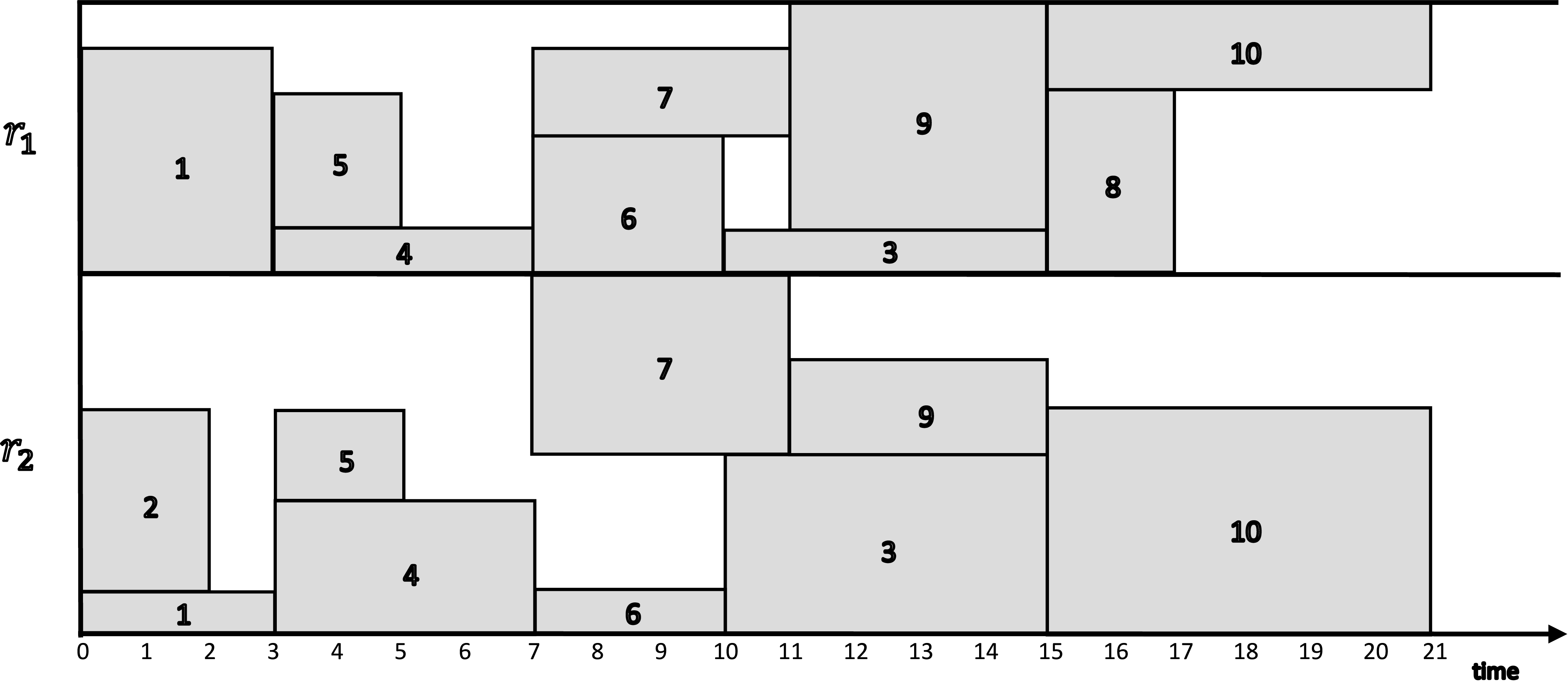
It is noteworthy that this particular problem instance has multiple optimal solutions. Keep in the mind that the solver may obtain a different optimum solution.

Job Shop Scheduling Problem

The Job Shop Scheduling Problem (JSSP) is an NP-hard problem defined by a set of jobs that must be executed by a set of machines in a specific order for each job. Each job has a defined execution time for each machine and a defined processing order of machines. Also, each job must use each machine only once. The machines can only execute a job at a time and once started, the machine cannot be interrupted until the completion of the assigned job. The objective is to minimize the makespan, i.e. the maximum completion time among all jobs.

For instance, suppose we have 3 machines and 3 jobs. The processing order for each job is as follows (the processing time of each job in each machine is between parenthesis):

• Job \(j_1\): \(m_3\) (2) \(\rightarrow\) \(m_1\) (1) \(\rightarrow\) \(m_2\) (2)
• Job \(j_2\): \(m_2\) (1) \(\rightarrow\) \(m_3\) (2) \(\rightarrow\) \(m_1\) (2)
• Job \(j_3\): \(m_3\) (1) \(\rightarrow\) \(m_2\) (2) \(\rightarrow\) \(m_1\) (1)

Bellow there are two feasible schedules:

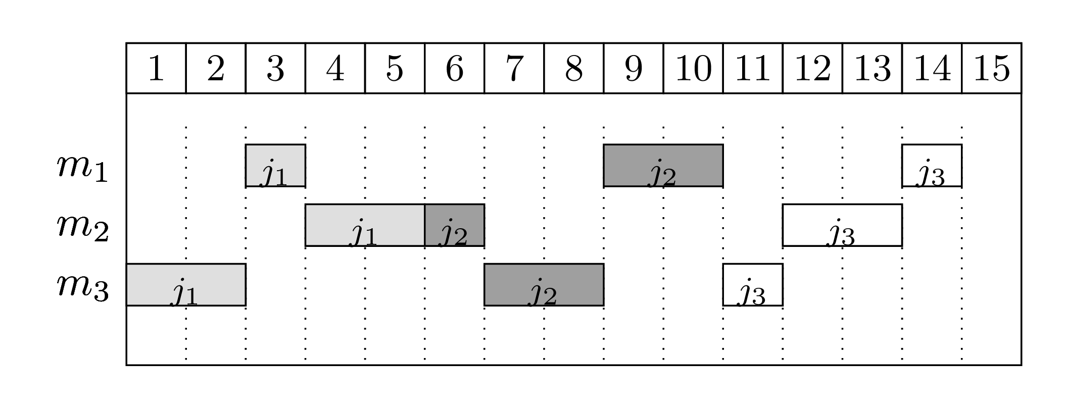
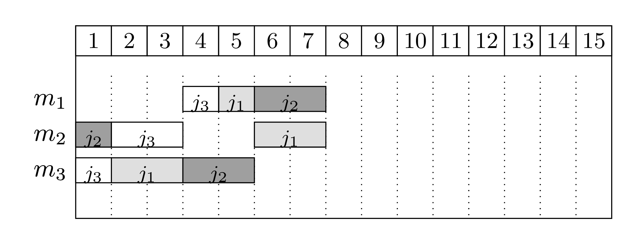
The first schedule shows a naive solution: jobs are processed in a sequence and machines stay idle quite often. The second solution is the optimal one, where jobs execute in parallel.

The JSSP has the following input data:

\(\mathcal{J}\)

set of jobs, \(\mathcal{J} = \{1,...,n\}\),

\(\mathcal{M}\)

set of machines, \(\mathcal{M} = \{1,...,m\}\),

\(o^j_r\)

the machine that processes the \(r\)-th operation of job \(j\), the sequence without repetition \(O^j = (o^j_1,o^j_2,...,o^j_m)\) is the processing order of \(j\),

\(p_{ij}\)

non-negative integer processing time of job \(j\) in machine \(i\).

A JSSP solution must respect the following constraints:

• All jobs \(j\) must be executed following the sequence of machines given by \(O^j\),
• Each machine can process only one job at a time,
• Once a machine starts a job, it must be completed without interruptions.

The objective is to minimize the makespan, the end of the last job to be executed. The JSSP is NP-hard for any fixed \(n \ge 3\) and also for any fixed \(m \ge 3\).

The decision variables are defined by:

\(x_{ij}\)

starting time of job \(j \in J\) on machine \(i \in M\)

\(y_{ijk}=\)

\(\begin{cases} 1, & \text{if job } j \text{ precedes job } k \text{ on machine } i \text{,}\\ & i \in \mathcal{M} \text{, } j, k \in \mathcal{J} \text{, } j \neq k \\ 0, & \text{otherwise} \end{cases}\)

\(C\)

variable for the makespan

Follows a MIP formulation [Mann60] for the JSSP. The objective function is computed in the auxiliary variable \(C\). The first set of constraints are the precedence constraints, that ensure that a job on a machine only starts after the processing of the previous machine concluded. The second and third set of disjunctive constraints ensure that only one job is processing at a given time in a given machine. The \(M\) constant must be large enough to ensure the correctness of these constraints. A valid (but weak) estimate for this value can be the summation of all processing times. The fourth set of constrains ensure that the makespan value is computed correctly and the last constraints indicate variable domains.

\[\begin{split}\textrm{Minimze: } \;\;\; & C \\ \textrm{Suject to: } \;\;\; & x_{o^{j}_{r},j} \geq x_{o^{j}_{r-1},j} +p_{o^{j}_{r-1},j} \,\,\, &\forall r \in \{2,..,m\}, j \in \mathcal{J} \\ & x_{i,j} \geq x_{i,k} + p_{i,k} - M \cdot y_{i,j,k} \,\,\, &\forall j,k \in \mathcal{J}, j \neq k, i \in \mathcal{M} \\ & x_{i,k} \geq x_{i,j} + p_{i,j} - M \cdot (1-y_{i,j,k}) \,\,\, &\forall j,k \in \mathcal{J}, j \neq k,i \in \mathcal{M} \\ & C \geq x_{o^{j}_{m},j} + p_{o^{j}_{m},j} \,\,\, &\forall j \in \mathcal{J} \\ & x_{i,j} \geq 0 \,\,\, &\forall i \in \mathcal{J}, i \in \mathcal{M} \\ & y_{i,j,k} \in \{0,1\} \,\,\, &\forall j,k \in \mathcal{J}, i \in \mathcal{M}\end{split}\]

The following Kotlin-MIP code creates the previous formulation, optimizes it and prints the optimal solution found:

Cutting Stock / One-dimensional Bin Packing Problem

The One-dimensional Cutting Stock Problem (also often referred to as One-dimensional Bin Packing Problem) is an NP-hard problem first studied by Kantorovich in 1939 [Kan60]. The problem consists of deciding how to cut a set of pieces out of a set of stock materials (paper rolls, metals, etc.) in a way that minimizes the number of stock materials used.

[Kan60] proposed an integer programming formulation for the problem, given below:

\[\begin{split}\textrm{min:} & \sum_{j=1}^{n} y_{j} \\ \textrm{s.t.:} & \sum_{j=1}^{n} x_{i,j} \geq b_{i} \;\; \forall i \in \{ 1 \ldots m \} \\ & \sum_{i=1}^{m} w_{i}x_{i,j} \leq L y_{j} \;\; \forall j \in \{ 1 \ldots n \} \\ & y_{j} \in \{0,1\} \;\; \forall j\in \{1 \ldots n\} \\ & x_{i,j} \in \mathbb{Z}^+ \;\; \forall i\in \{1 \ldots m\}, \forall j\in \{1 \ldots n\}\end{split}\]

This formulation can be improved by including symmetry reducing constraints, such as:

\[\begin{split}y_{j-1} \geq y_{j} \;\; \forall j \in \{ 2 \ldots m \} \\\end{split}\]

The following Kotlin-MIP code creates the formulation proposed by [Kan60], optimizes it and prints the optimal solution found.

Two-Dimensional Level Packing

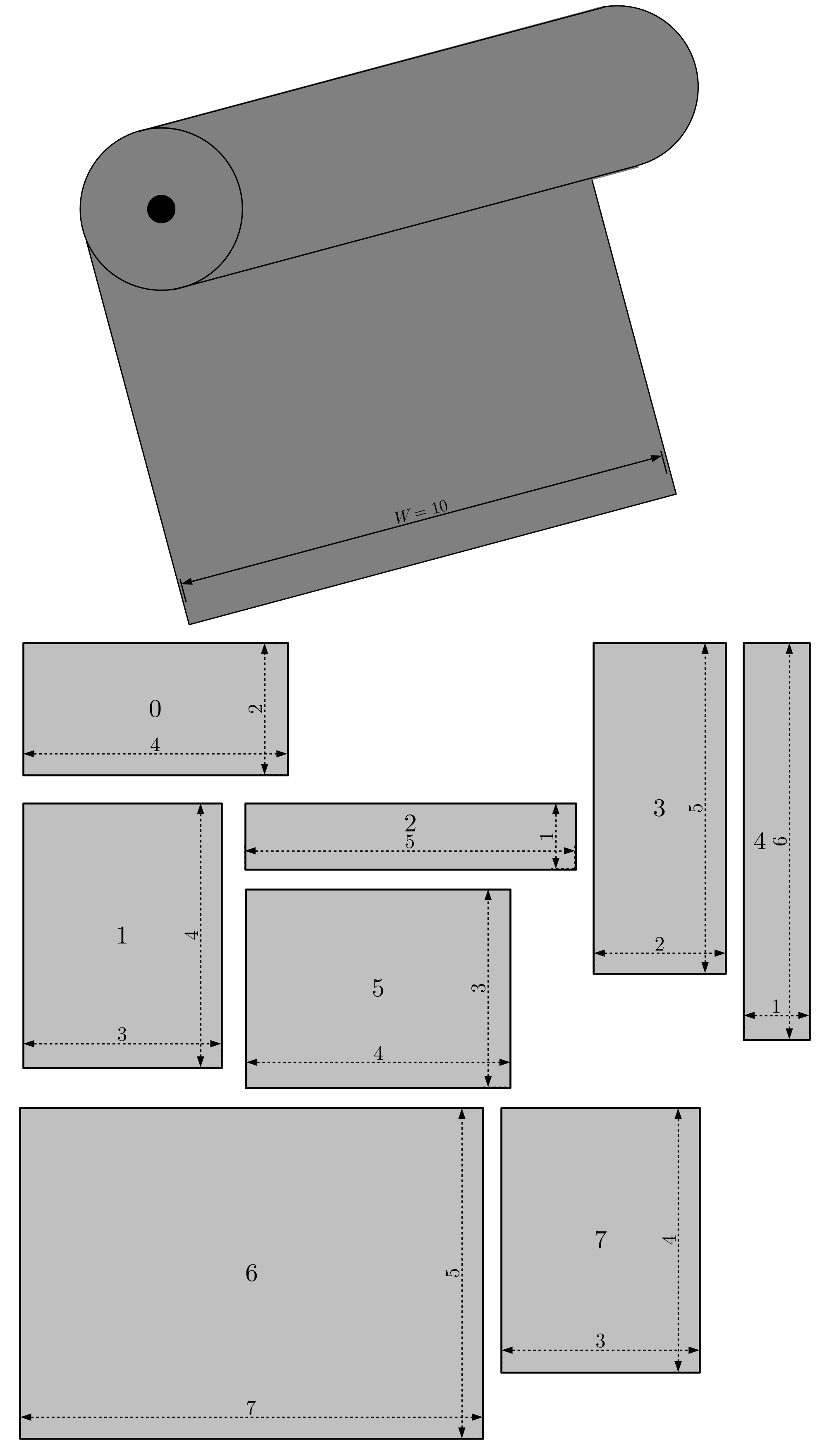
In some industries, raw material must be cut in several pieces of specified size. Here we consider the case where these pieces are rectangular [LMM02]. Also, due to machine operation constraints, pieces should be grouped horizontally such that firstly, horizontal layers are cut with the height of the largest item in the group and secondly, these horizontal layers are then cut according to items widths. Raw material is provided in rolls with large height. To minimize waste, a given batch of items must be cut using the minimum possible total height to minimize waste.

Formally, the following input data defines an instance of the Two Dimensional Level Packing Problem (TDLPP):

\(W\)

raw material width

\(n\)

number of items

\(I\)

set of items = \(\{0, \ldots, n-1\}\)

\(w_i\)

width of item \(i\)

\(h_i\)

height of item \(i\)

The following image illustrate a sample instance of the two dimensional level packing problem.

This problem can be formulated using binary variables \(x_{i,j} \in \{0, 1\}\), that indicate if item \(j\) should be grouped with item \(i\) (\(x_{i,j}=1\)) or not (\(x_{i,j}=0\)). Inside the same group, all elements should be linked to the largest element of the group, the representative of the group. If element \(i\) is the representative of the group, then \(x_{i,i}=1\).

Before presenting the complete formulation, we introduce two sets to simplify the notation. \(S_i\) is the set of items with width equal or smaller to item \(i\), i.e., items for which item \(i\) can be the representative item. Conversely, \(G_i\) is the set of items with width greater or equal to the width of \(i\), i.e., items which can be the representative of item \(i\) in a solution. More formally, \(S_i = \{j \in I : h_j \leq h_i\}\) and \(G_i = \{j \in I : h_j \geq h_i\}\). Note that both sets include the item itself.

\[\begin{split}\textrm{min:} & \sum_{i \in I} x_{i,i} \\ \textrm{s.t.:} & \sum_{j \in G_i} x_{i,j} = 1 \;\; \forall i \in I \\ & \sum_{j \in S_i : j \neq i} x_{i,j} \leq (W-w_i)\cdot x_{i,i} \;\; \forall i \in I \\ & x_{i,j} \in \{0,1\} \;\; \forall (i,j) \in I^2\end{split}\]

The first constraints enforce that each item needs to be packed as the largest item of the set or to be included in the set of another item with width at least as large. The second set of constraints indicates that if an item is chosen as representative of a set, then the total width of the items packed within this same set should not exceed the width of the roll.

The following Kotlin-MIP code creates and optimizes a model to solve the two-dimensional level packing problem illustrated in the previous figure.

Plant Location with Non-Linear Costs

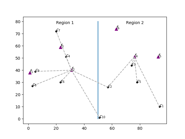
One industry plans to install two plants, one to the west (region 1) and another to the east (region 2). It must decide also the production capacity of each plant and allocate clients with different demands to plants in order to minimize shipping costs, which depend on the distance to the selected plant. Clients can be served by facilities of both regions. The cost of installing a plant with capacity \(z\) is \(f(z)=1520 \log z\). The Figure below shows the distribution of clients in circles and possible plant locations as triangles.

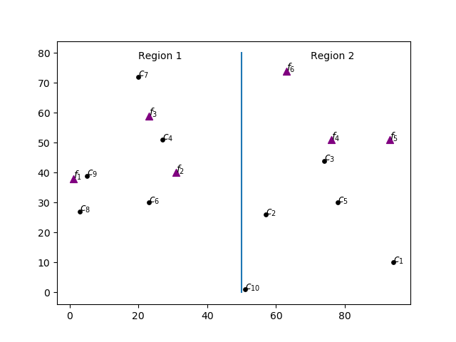
This example illustrates the use of Special Ordered Sets (SOS). We’ll use Type 1 SOS to ensure that only one of the plants in each region has a non-zero production capacity. The cost \(f(z)\) of building a plant with capacity \(z\) grows according to the non-linear function \(f(z)=1520 \log z\). Type 2 SOS will be used to model the cost of installing each one of the plants in auxiliary variables \(y\).

The allocation of clients and plants in the optimal solution is shown bellow. This example uses Matplotlib to draw the Figures.